Bipin's Bubble
Deep Kalman Filters
This is another paper in state estimation of Dynamic system. An earlier post on Variational RNN is a related approach to solve this issue.
This is a paper summary and notes written by me during reading this paper. I claim no rights to any intellectual property in this post. I am sharing this mostly for personal purposes and just in case someone might find my personal notes helpful
Introduction
This post is based on the paper: Deep Kalman Filters by Krishnan et. al. This paper was published in Advances in Approximate Bayesian Inference, NeurlIPS 2015.
The main goal of this paper is to model a dynamic system, e.g. a time series which has been motivated by counterfactual inference.
As usual, for sequence of observations $x_1, x_2, …, x_t$ assumed to be generated from some underlying latent process of $z_1, z_2, …, z_t$, Kalman Filters are used to model the dynamic latent system that governs how the latent variable dynamics changes with time and also simultaneously causes or generates the observations x.
The fundamental Kalman assumption is generally noted as:
\[z_t = \mathbf{G}_t z_{t-1} + \mathbf{B}_t u_{t-1} + \epsilon_t \\ x_t = \mathbf{F} z_t + \eta_t \\ where, \\ \epsilon_t \sim \mathcal{N} (0, \Sigma_t) \\ \eta_t \sim \mathcal{N} (0, \Gamma_t) \\\]Here we can see that the Kalman filter assumes that the latent state characterized by random variable $z$ transitions linearly with previous state and activations along with some stochastic noise. The observation $x$ is then just a linear function of state at same time instance and some additive noise, this function is called emission.
The algorithm suggested in the paper by Krishnan et. al, can be generalized to cases where both the transition and emission are not linear functions. However, for simplicity, this blog only focusses on the case for linearity, learning non linear function through Neural networks instead of linear functions should be trivial by gradient descent algorithms.
Modelling assumptions
This algorithm focusses mostly on transition functions and is claimed that it works for any parameteric distribution in for emission probability. The priors in latent spaces are therefore assumed as:
\[z_1 \sim \mathcal{N} (\mu_0, \Sigma_0) \\ z_t \sim \mathcal{N} (\ \mathbf{G}_\alpha (z_{t-1}, u_{t-1}), \ \mathcal{S}_\beta(z_{t-1}, u_{t-1}) \ ) \\ x_t \sim \Pi (\mathbf{F}_\kappa(z_t))\]- Where $\Pi$ can be any distribution.
- Latent varaibles are considered to be normally distributed with mean and function depending on previous state as well as input (based on Kalman Assumption above)
The graphical model for the assumption can be seen as:
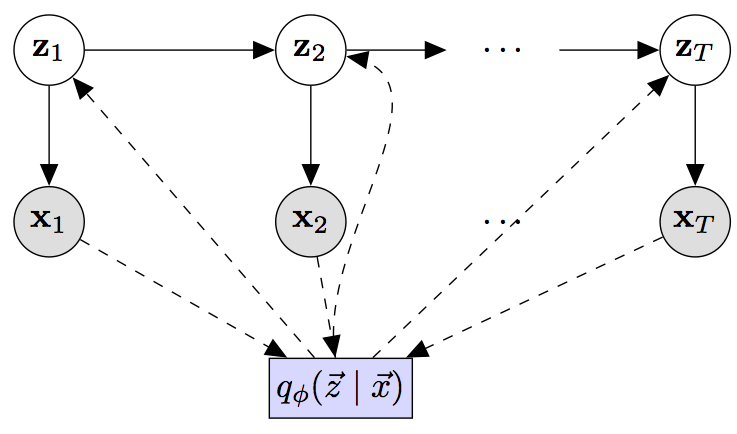
This figure has been taken from Github Implementation for a slightly different paper: Structured Inference Networks for Nonlinear State Space Models, AAAI 2017 by Krishan et al. The link to github is: clinicalml / structuredinference
based on the graphical model, we can factorize the approximate posterior for encoder as:
\[q_\phi(\vec{z} | \vec{x}, \vec{u}) = \prod_{t=1}^T q(z_t|z_{t-1}, x_t,..., x_T, \vec{u})\]Learning
Variational Inference can be used to learn this model. The evidence lower bound (ELBO) can be found as:
\[\begin{align} log \ p(\vec{x} | \vec{u}) &= log \int p(\vec{x}, \ \vec{z} \ | \ \vec{u}) \ d\vec{z} \\ &= log \int p(\vec{x}, \ \vec{z} \ | \ \vec{u}) * \dfrac{q(\vec{z} | \vec{x}, \vec{u})}{q(\vec{z} | \vec{x}, \vec{u})} \ d\vec{z} \\ &\ge \int q_\phi(\vec{z} | \vec{x}, \vec{u}) * log(\dfrac{p(\vec{x}, \ \vec{z} \ | \ \vec{u})}{q_\phi(\vec{z} | \vec{x}, \vec{u})}) \end{align}\]which is the ELBO.
The ELBO further reduces to:
\[\begin{align} \mathcal{L} &= \int q_\phi(\vec{z} | \vec{x}, \vec{u}) * log(\dfrac{p(\vec{x}, \ \vec{z} \ | \ \vec{u})}{q_\phi(\vec{z} | \vec{x}, \vec{u})}) \\ &= E_{enc}[log(\dfrac{p(\vec{x}, \ \vec{z} \ | \ \vec{u})}{q_\phi(\vec{z} | \vec{x}, \vec{u})}] \\ &= E_{enc}[log(\dfrac{p(\vec{x}, \ | \ \vec{z} \ \vec{u}) * p(\vec{z} | \vec{u})}{q_\phi(\vec{z} | \vec{x}, \vec{u})})] \\ &= E_{enc}[log \ p(\vec{x} \ | \ \vec{z} \ \vec{u}) + log(\dfrac{ p(\vec{z} | \vec{u})}{q_\phi(\vec{z} | \vec{x}, \vec{u})})] \\ &= E_{enc}[log \ p(\vec{x} \ | \ \vec{z}, \ \vec{u})] - KL( q_\phi(\vec{z} | \vec{x}, \vec{u}) || p(\vec{z} | \vec{u}||)) \end{align}\]The two terms in ELBO can further be simplified further as:
\[\begin{align} E_{enc}[log \ p(\vec{x} \ | \ \vec{z}, \ \vec{u})] &= E_{enc}[log \prod_{t=1}^T p(x_t | z_t, u_{t-1})] \\ &= E_{enc}[\sum_{t=1}^T log \ p(x_t | z_t, u_{t-1})] \\ &= \sum_{t=1}^T E_{enc}[ log \ p(x_t | z_t, u_{t-1})] \\ \end{align}\]AND,
\[\begin{align} KL( q_\phi(\vec{z} | \vec{x}, \vec{u}) || p(\vec{z} | \vec{u}||)) &= \int q_\phi(\vec{z} | \vec{x}, \vec{u}) * log \ \dfrac{p(\vec{z} | \vec{u})}{q_\phi(\vec{z} | \vec{x}, \vec{u})} \ d\vec{z} \\ &= E_{enc}[log \ \dfrac{p(\vec{z} | \vec{u})}{q_\phi(\vec{z} | \vec{x}, \vec{u})}] \\ &= E_{enc}[log \ \dfrac{\prod_{t=1}^T p(z_t | z_{t-1}, \vec{u})}{\prod_{t=1}^T q(z_t | z_{t-1}, \vec{x}, \vec{u})}]\\ &= E_{enc}[log \ \prod_{t=1}^T \dfrac{ p(z_t | z_{t-1}, \vec{u})}{ q(z_t | z_{t-1}, \vec{x}, \vec{u})}] \\ &= E_{enc}[log \ \prod_{t=2}^T \dfrac{ p(z_t | z_{t-1}, \vec{u})}{ q(z_t | z_{t-1}, \vec{x}, \vec{u})} + log \dfrac{p(z_1|z_0)}{q(z_1|z_0, \vec{x})}] \\ &= E_{enc}[log \ \prod_{t=2}^T \dfrac{ p(z_t | z_{t-1}, \vec{u})}{ q(z_t | z_{t-1}, \vec{x}, \vec{u})}] + E_{enc}[log \dfrac{p(z_1|z_0)}{q(z_1|z_0, \vec{x})}] \\ &= E_{enc}[\sum_{t=2}^T log \ \dfrac{ p(z_t | z_{t-1}, \vec{u})}{ q(z_t | z_{t-1}, \vec{x}, \vec{u})}] + E_{enc}[log \dfrac{p(z_1)}{q(z_1|\vec{x})}] \\ &= \sum_{t=2}^T E_{enc}[log \ \dfrac{ p(z_t | z_{t-1}, \vec{u})}{ q(z_t | z_{t-1}, \vec{x}, \vec{u})}] + E_{enc}[log \dfrac{p(z_1)}{q(z_1|\vec{x})}] \\ &= \sum_{t=2}^T E[KL(q(z_t | z_{t-1}, \vec{x}, \vec{u})) \ || \ p(z_t | z_{t-1}, \vec{u})] + \\ & KL(q(z_1|\vec{x}) || p(z_1)) \\ \end{align}\]The combined loss function (negative ELBO) thus obtained can be optimized and thus the model can be learnt.
The ELBo optimizes KL between prior on latent variable z and the encoder function, i.e. the optimal is when encoder can encode close to prior, so what this algorithm is actually doing is learning a way to correctly encode the latent variable given observations.
This model can be used for state estimation of dynamic systems characterized by non-linear Kalman Latent Process.
References
- [1] R. G. Krishnan, U. Shalit, and D. Sontag, “Deep Kalman Filters.” arXiv, Nov. 25, 2015. Accessed: Sep. 07, 2022. [Online]. Available: http://arxiv.org/abs/1511.05121
- [2] Image for the Graphical model taken from clinicalml’s github:
clinicalml/structuredinference